Title: Modelling Mass Balance and Flow Dynamics of Haut Glacier d’Arolla Under Historical and Projected Climate Forcing

Abstract: This study develops a physically realistic model of Haut Glacier d’Arolla by incorporating basal sliding into a flowline–mass balance framework. Calibration against historical geometry and surface velocities identified a best-fit parameter set, establishing a reliable basis for further analysis. Climate sensitivity tests revealed that temperature is the dominant control on glacier evolution, while precipitation had a smaller, nonlinear effect. Future projections based on three GCMs and RCP scenarios indicate near-complete glacier loss by 2100, even under RCP2.6. Inter-GCM variability accounts for most of the projection spread, far exceeding the effect of internal model uncertainties. These results highlight the vulnerability of small Alpine glaciers to warming, and the importance of glacier-specific, calibrated models with downscaled climate inputs for improving impact assessments in mountain regions.

1. Introduction

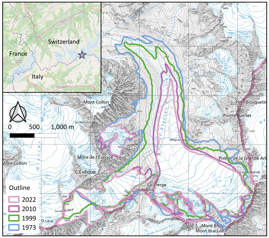
About one-third of projected sea-level rise over the next century will result from the melt of valley glaciers and small ice caps (Warrick et al., 1996), necessitating the understanding of these glacier systems. Haut Glacier d’Arolla, located in the western Pennine Alps, Switzerland, offers an ideal case due to its simple geometry, small size, and high ice flux (Hubbard et al., 1998; Figure 1). The glacier is ~4 km long, and has undergone significant shrinking, from 6.3 km² in 1998 to 3.3 km² by 2023 (Dadic, Corripio and Burlando, 2008; Shaw et al., 2023). Previous research of this glacier focused on sediment transport (Swift et al., 2011), meltwater chemistry (Brown et al., 1994), and hydrology (Nienow, Sharp and Willis, 1998; Willis et al., 2003). High-resolution flow models were also applied (Hubbard et al., 1998), but were not used to simulate long-term evolution or tested against observations. Moreover, no studies have implemented climate sensitivity tests or GCM-forced projections at Haut Glacier d’Arolla. These approaches have been widely applied to other Alpine glaciers (Wallinga and Wal, 1998; Anderson, Lawson and Owens, 2008) to assess future glacier responses.

This study addresses these gaps with a mass balance–flowline model, aiming to:

1. Choose physically realistic flow parameters that can reproduce observed geometry when forced with historical climate (1930-1990);

2. Assess glacier sensitivity to temperature and precipitation perturbations under a pre-warming climatological baseline (1960–1990);

3 Simulate future glacier evolution under multiple GCM–RCP scenarios and quantify projection uncertainty.

2. Method

2.1 Model

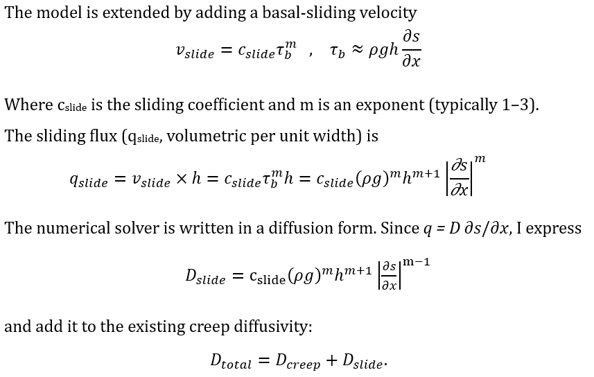
This project builds on a glacier model provided by the Department, which combines Glen’s flow law with a Positive Degree Day mass balance scheme (Braithwaite and Zhang, 2000). However, the original model simulates ice velocity through deformation alone, omitting basal sliding—a key process in temperate glaciers (Hubbard et al., 1998). To address this, I incorporated a Weertman-type sliding law to the model: \(v_{\text{slide}} = c_{\text{slide}} \, \tau_b^m\) Where c is the sliding coefficient, m is an exponent, and τ is the basal shear stress. This modification enables more realistic flow simulations and allows focused assessment of basal dynamics under different climate and parameter conditions. Scripts are provided in the appendix.

Question 1

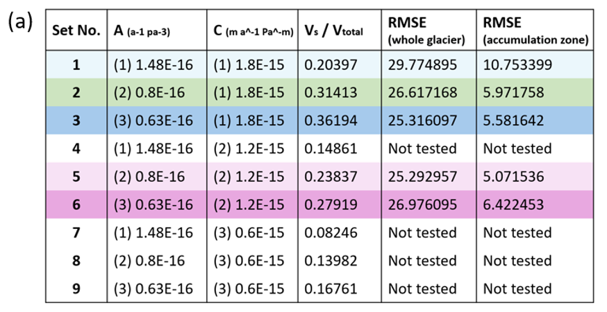
This section aims to identify the best flow-law parameter sets. A 3×3 matrix of candidate parameter sets was generated, with three creep coefficients (A) and three sliding coefficients (c). The justification for each value is provided in Table 1. The flow-law exponents were fixed (n = 3, m = 3), following Hubbard et al. (1998), as these values are well established in glacier modelling (Weertman, 1957; Gilbert et al., 2023).

There were two phases of tests. The first phase assessed whether each parameter set produced physically realistic ice dynamics by evaluating the contribution of basal sliding to total surface velocity. Simulations were run for three years under constant 1930 climate forcing with 1930 geometry. At each timestep, surface velocities were decomposed into deformational and sliding components, then averaged longitudinally and over time. As no annual velocity data exist for Haut Glacier d’Arolla, I adopted a benchmark from Morteratsch Glacier, where sliding contributes ~30% of the annual surface velocity (Zekollari et al., 2013). Parameter sets yielding sliding fractions between 20–40% were considered physically plausible and retained for further testing.

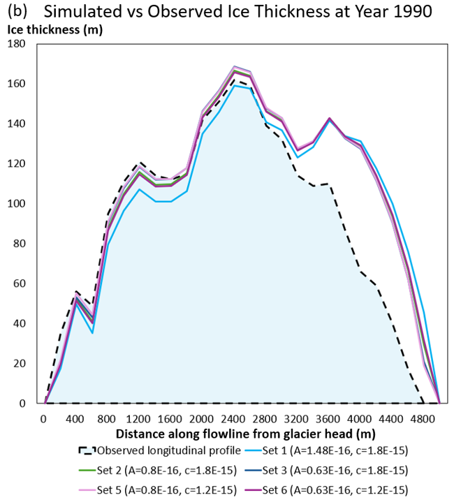
The second phase tests the ability to reproduce historical observations. Models were forced with transient 1930-1990 climate data, and the simulated geometry in 1990 were evaluated against observation with two metrics: (1) deviation of total glacier length, and (2) root-mean-square error (RMSE) of thickness along the glacier centreline. The set with best performance in both tests was used for the following sensitivity test and GCM-based prediction.

Question 2

To assess the glacier’s climatic sensitivity, I performed stepwise perturbation experiments on temperature and precipitation relative to the 1960–1990 climatological mean, using fixed 1990 geometry. This period is widely adopted as a pre-accelerated-warming benchmark in glacier sensitivity studies (Oerlemans, 1992, 1997a; Zekollari, Huss and Farinotti, 2019), ensuring comparability with previous studies.

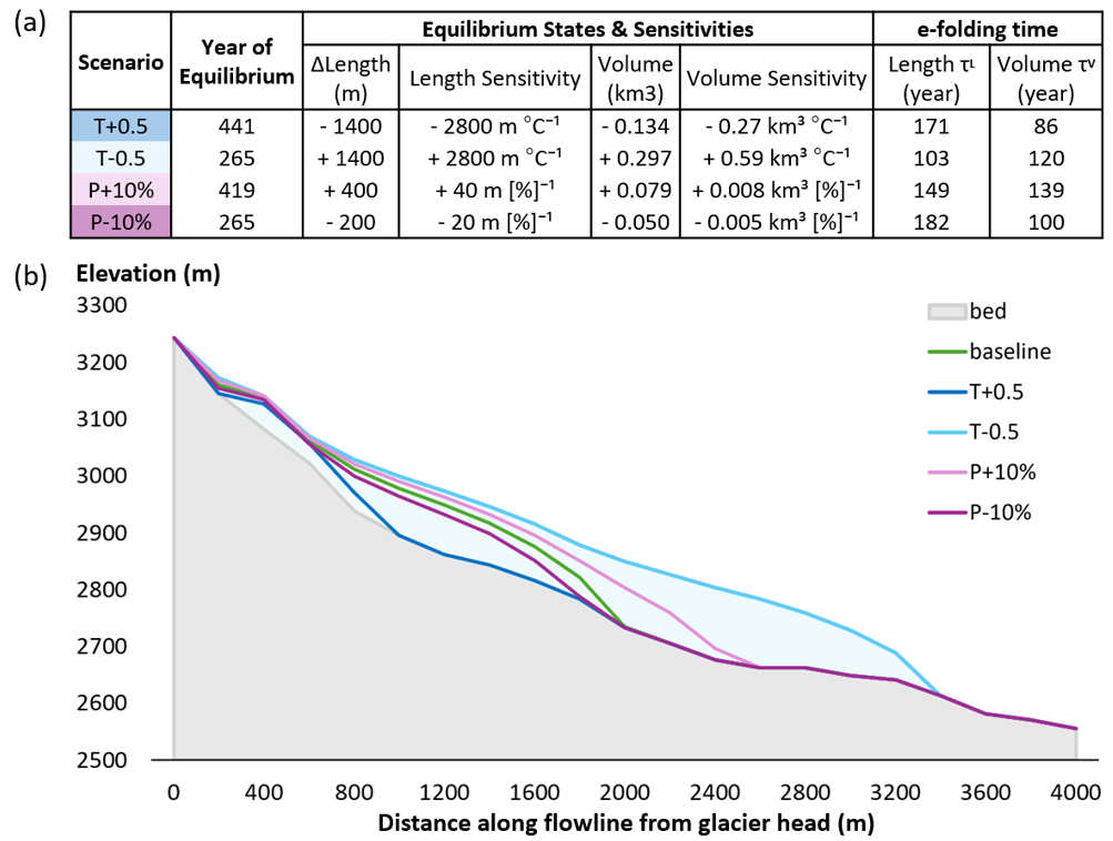
Initial tests applied standard perturbations of ±1 °C and ±10 % precipitation (Oerlemans and Fortuin, 1992; Braithwaite and Zhang, 2000). However, under +1 °C, the glacier fully melted before reaching equilibrium, invalidating steady-state sensitivity metrics such as ΔV/ΔT. I therefore refined the experiment to use smaller ±0.5 °C temperature steps, while keeping ±10 % precipitation perturbations.

Equilibrium was rigorously defined following OGGM protocols (Maussion et al., 2019): (1) the 60-year running mean of net mass balance remained within ±0.05 m w.e. a⁻¹, and (2) year-on-year relative volume change was below 0.1 % a⁻¹. Both thresholds had to persist for ≥30 years to avoid transient effects.

Sensitivity was quantified by comparing the equilibrium glacier length and volume against the baseline. Additionally, I computed the e-folding time constant (τ)—the time taken for the glacier to achieve ~63% of its total adjustment after a perturbation (Jóhannesson, Raymond and Waddington, 1989) to evaluate response timescales.

Question 3

The best-fit parameter set was used to project glacier evolution under climate forcing from three General Circulation Models (CCSM4, CGCM3, HadGEM2) across RCP2.6, 4.5, and 8.5 scenarios. RCPs (Representative Concentration Pathways) describe varying greenhouse gas trajectories, with values corresponding to radiative forcing levels (W/m²) by 2100 (IPCC, 2013). To assess the relative influence of climate uncertainty versus structural model uncertainty, I ran an additional ensemble using CCSM4 forcing with ±20% perturbations to the creeping and sliding coefficients, and compared the spread in projected glacier length and volume.

3. Results

Question 1

Five of nine parameter sets met the physically plausible basal sliding ratio (Vs/Vtotal) of 20–40% (Figure 2a). Sets with the lowest sliding coefficient (Sets 7–9) and one mid-range set (Set 4) fell below this threshold (≤17%), while none exceeded 40%. All retained sets reproduced the observed 1990 glacier length (~4800 m) under 1930–1990 forcing. Thickness profiles in the accumulation zone were well captured (RMSE: 5.1–10.8 m, <10% of average thickness), but all sets overestimated thickness in the ablation zone, increasing the RMSE for the full glacier profile to 25–30 m. Set 5 yielded the lowest RMSE for both the accumulation zone (5.07 m) and the full profile (25.29 m), and was selected for subsequent experiments. However, Set 3 performed comparably, suggesting equifinality within the calibrated parameter space (Figure 2b). 

Question 2

Overall, the model yields a length sensitivity of 2800 m °C⁻¹ and a volume sensitivity of 0.43 km³ °C⁻¹. Sensitivity to precipitation is lower, 0.3 km in length and ±0.06 km³ in volume per 10% change (Figure 5). Length has symmetric response to temperature (±2800 m °C⁻¹), but asymmetric for precipitation (+300 m vs. –100 m per 10%). Volume response is more asymmetric: gains from cooling (+0.59 km³ °C⁻¹) exceed losses from warming (–0.27 km³ °C⁻¹), and increases due to precipitation (+0.079 km³) exceed losses from it (–0.050 km³). E-folding times reveal that length adjusts faster under advance scenarios, whereas volume responds faster under retreat scenarios.

Question 3

As figure 4 presents, simulated volume declines rapidly before mid-century and then stabilizes; length responds more slowly at first but undergoes accelerated retreat after ~2050. Inter-model spread is substantial: CGCM3 projects the slowest ice loss, HadGEM2 the fastest, with CCSM4 intermediate. Ensemble means show ice persisting under RCP2.6 until ~2100, while RCP4.5 and 8.5 reach near-zero volume by ~2080 and ~2070, respectively. Notably, ensemble averaging masks late-century nonlinearity—particularly the consistent post-2050 acceleration in glacier length retreat across all GCMs.

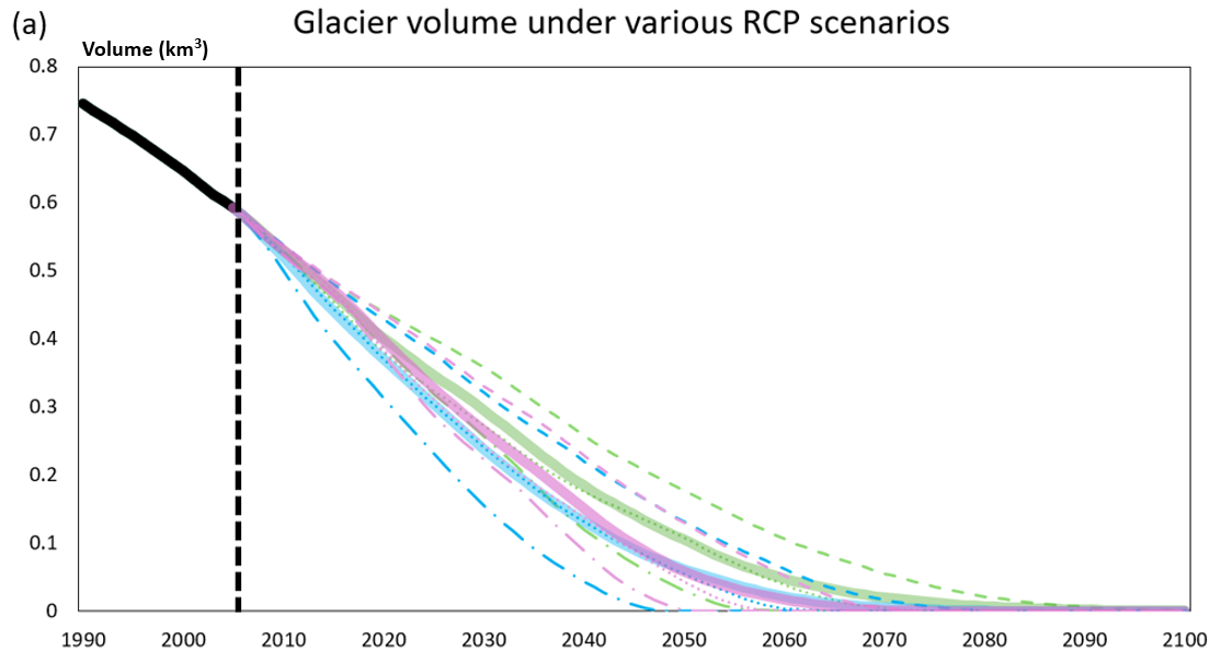
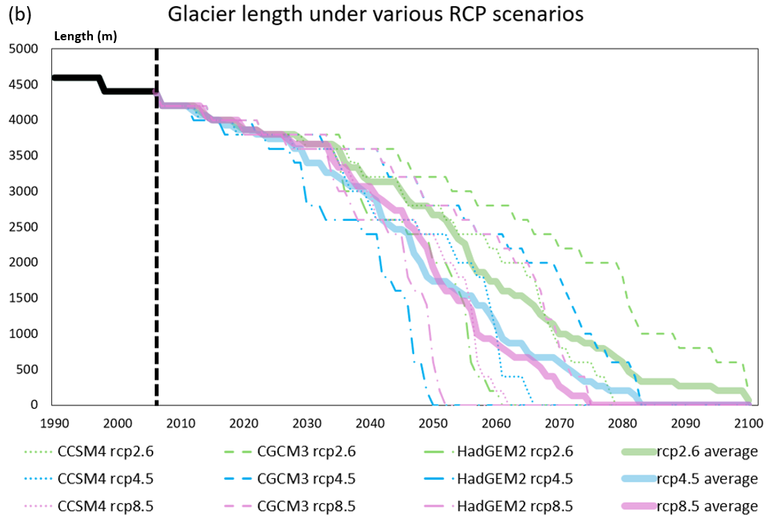
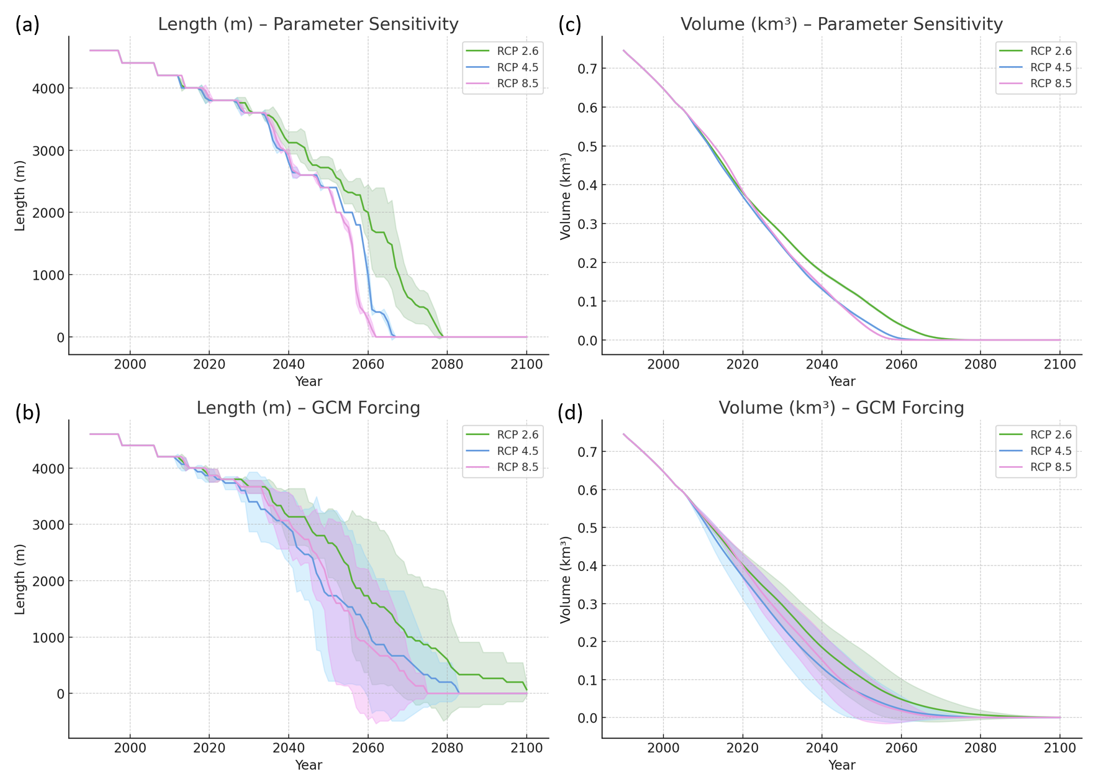
Figure 5 shows that perturbing the deformation and sliding coefficients (±20%) produces minimal spread in projected volume and length, especially under RCP4.5/8.5. In contrast, inter-GCM spread is an order of magnitude larger, with substantial overlap in trajectory bands even across different RCPs. These results demonstrate that uncertainty in climate forcing, not parameter calibration, is the dominant source of projection variability in future glacier evolution.

4. Discussion

Question 1

The best-fit parameter set has a flow coefficient of A = 0.8 × 10⁻¹⁶ Pa⁻³ a⁻¹, consistent with published values for temperate ice (e.g., Cuffey and Paterson, 2010). It is slightly higher than the winter-specific estimate for Haut Glacier d’Arolla (A = 0.63 × 10⁻¹⁶ Pa⁻³ a⁻¹, Hubbard et al., 1998), likely reflecting enhanced summer deformation due to higher temperatures. The sliding coefficient (C = 1.2 × 10⁻¹⁵ Pa⁻³ m² a⁻¹) matches the best-fit value reported for Morteratsch Glacier (Zekollari et al., 2013), suggesting regional consistency. The systematic over-thickening in the ablation zone likely arises from structural, rather than parametric, uncertainty. One probable cause is the use of a spatially uniform degree-day factor (DDF). In reality, DDF increases downslope due to reduced albedo from supraglacial debris (Carenzo et al., 2016), representing higher melting rate at the glacier tongue. Incorporating a Debris-Enhanced Temperature-Index (DETI) scheme could improve ablation modeling. Another explanation for the systematic error might raise from the assumption of static flowline geometry from 1930–1990. In reality, flowline shifts and width variations can affect cross-sectional flow, and should be further investigated using historical maps or DEM reconstructions.

The model illustrates the well-known equifinality problem in glaciology, where multiple parameter sets produce similarly acceptable fits (Enderlin et al. 2013; Zeitz et al., 2020). Addressing this may require multi-criteria calibration, e.g., incorporating width, strain rates, or velocity profiles. Meanwhile, while this study used classical exponents (n = m = 3), recent experiments suggest n ≈ 1 for temperate ice (Schohn et al., 2025) and sub-linear or Coulomb-style basal sliding laws for hard beds (e.g., Zoet and Iverson, 2020). Future work could explore these alternatives using Bayesian or ensemble frameworks to constrain deeper model uncertainty.

Question 2

Sensitivity tests confirm that temperature is the dominant driver of glacier evolution, with precipitation playing a secondary role—consistent with findings for other Alpine and temperate glaciers (e.g., Che et al., 2019; Kinnard et al., 2022). This is expected, as a 1 °C warming requires a ~20–35% increase in precipitation to offset enhanced melt (Oerlemans, 1981; Raper et al., 2000).

My model yields a length sensitivity of 2.8 km K⁻¹, closely matching Franz Josef Glacier’s 2.7 km K⁻¹ (Anderson et al., 2008). However, volume sensitivity is lower (0.43 km³ K⁻¹ vs. 1.6 km³ K⁻¹ in Anderson et al.), suggesting underestimation of ice-thickness change. Precipitation sensitivities are slightly lower than Oerlemans (1997b), yet within a comparable range (e.g., 0.3 km length per 10% vs. 0.5 km; 0.06 km³ volume vs. 0.9 km³), indicating realistic but moderately conservative model behavior.

The asymmetry in response time—fast volume loss under warming, slow regrowth under cooling—is common in the European Alps, since thinning can happen rapidly at low elevations while thickening in the accumulation zone needs to advect through the whole flowline and therefore delays response (Zekollari et al., 2020). However, the reversed asymmetry in glacier length (faster advance than retreat) is atypical and may reflect nonlinear feedbacks or flowline-specific geometries, warranting further investigation.

Question 3

GCM-forced simulations project that Haut Glacier d’Arolla (HGA) will disappear by ~2095 even under the low-emission RCP2.6 scenario, indicating its high vulnerability compared to other Alpine glaciers. This aligns with projections from Zekollari et al. (2019), who estimated that only one-third of Alpine glacier volume will remain by 2100 under mitigation, and over 90% will be lost under high-emission scenarios. The relative severity of the three GCMs used (CGCM3 < CCSM4 < HadGEM2) mirrors broader assessments—HadGEM2 is consistently recognized for its warm bias (Huss and Hock, 2015).

The result supports the conclusion by Zekollari et al. (2019) that future glacier change is more strongly influenced by the choice of GCM than by internal model parameters. Moreover, as Marzeion et al., (2020) highlight, scenario uncertainty becomes the dominant source of projection spread by 2100. This underlines the growing value of glacier-specific modelling—especially for assessing localized impacts—which is emphasized in recent regional downscaling efforts (Zekollari et al., 2024).

5. Conclusion

This study advances glacier modelling by incorporating basal sliding into a flowline framework and calibrating it against observed velocity and geometry. The best-fit parameter set aligns with regional estimates, enhancing confidence in simulated dynamics. Sensitivity tests confirmed temperature as the dominant driver of glacier evolution, with length and volume exhibiting asymmetric sensitivities and response times. Assumptions like flowline constancy and uniform DDFs may introduce structural bias that warrant further investigation. Projections indicate near-total loss of Haut Glacier d’Arolla by 2100, even under RCP2.6. Inter-GCM variability far exceeds internal model uncertainties, demonstrating the need for downscaled, glacier-specific climate inputs.

Examiner feedback: 92/100, EEE, first class with distinction. “Comment: This is an excellent piece of work. The prose are clear throughout, and the author does a good job at justifying the importance of studying alpine valley glaciers. The study design is incredibly ambitious, as the author implements a basal sliding scheme into the code that they were provided. This demonstrates advanced conceptual and methodological understanding. The results and discussion were well written. It would have been nice to have been provided with more detail, but given the ambitions of the project, and the word limit, I can see that this wasn’t possible. Overall, this work was remarkable.”

6. Bibliography

Anderson, B., Lawson, W. and Owens, I. (2008) ‘Response of Franz Josef Glacier Ka Roimata o Hine Hukatere to climate change’, Global and Planetary Change, 63(1), pp. 23–30. Available at: https://doi.org/10.1016/j.gloplacha.2008.04.003.

Braithwaite, R.J. and Zhang, Y. (2000) ‘Sensitivity of mass balance of five Swiss glaciers to temperature changes assessed by tuning a degree-day model’, Journal of Glaciology, 46(152), pp. 7–14. Available at: https://doi.org/10.3189/172756500781833511.

Brown, G.H. et al. (1994) ‘Impact of post-mixing chemical reactions on the major ion chemistry of bulk meltwaters draining the haut glacier d’arolla, valais, Switzerland’, Hydrological Processes, 8(5), pp. 465–480. Available at: https://doi.org/10.1002/hyp.3360080509.

Carenzo, M. et al. (2016) ‘An enhanced temperature index model for debris-covered glaciers accounting for thickness effect’, Advances in Water Resources, 94, pp. 457–469. Available at: https://doi.org/10.1016/j.advwatres.2016.05.001.

Che, Y. et al. (2019) ‘Energy balance model of mass balance and its sensitivity to meteorological variability on Urumqi River Glacier No.1 in the Chinese Tien Shan’, Scientific Reports, 9(1), p. 13958. Available at: https://doi.org/10.1038/s41598-019-50398-4.

Cuffey, K. and Paterson, W.S.B. (2010) The physics of glaciers. 4th ed. Burlington, MA: Butterworth-Heinemann/Elsevier.

Dadic, R., Corripio, J.G. and Burlando, P. (2008) ‘Mass-balance estimates for Haut Glacier d’Arolla, Switzerland, from 2000 to 2006 using DEMs and distributed mass-balance modeling’, Annals of Glaciology, 49, pp. 22–26. Available at: https://doi.org/10.3189/172756408787814816.

Enderlin, E.M., Howat, I.M. and Vieli, A. (2013) ‘The sensitivity of flowline models of tidewater glaciers to parameter uncertainty’, The Cryosphere, 7(5), pp. 1579–1590. Available at: https://doi.org/10.5194/tc-7-1579-2013.

Gilbert, A. et al. (2023) ‘Inferring the Basal Friction Law From Long Term Changes of Glacier Length, Thickness and Velocity on an Alpine Glacier’, Geophysical Research Letters, 50(16), p. e2023GL104503. Available at: https://doi.org/10.1029/2023GL104503.

Hubbard, A. et al. (1998) ‘Comparison of a three-dimensional model for glacier flow with field data from Haut Glacier d’Arolla, Switzerland’, Journal of Glaciology, 44(147), pp. 368–378. Available at: https://doi.org/10.3189/S0022143000002690.

Huss, M. and Hock, R. (2015) ‘A new model for global glacier change and sea-level rise’, Frontiers in Earth Science, 3. Available at: https://www.frontiersin.org/articles/10.3389/feart.2015.00054 (Accessed: 13 February 2024).

Jóhannesson, T., Raymond, C.F. and Waddington, E.D. (1989) ‘A Simple Method for Determining the Response Time of Glaciers’, in J. Oerlemans (ed.) Glacier Fluctuations and Climatic Change. Dordrecht: Springer Netherlands, pp. 343–352. Available at: https://doi.org/10.1007/978-94-015-7823-3_22.

Kinnard, C. et al. (2022) ‘Modelling glacier mass balance and climate sensitivity in the context of sparse observations: application to Saskatchewan Glacier, western Canada’, The Cryosphere, 16(8), pp. 3071–3099. Available at: https://doi.org/10.5194/tc-16-3071-2022.

Marzeion, B. et al. (2020) ‘Partitioning the Uncertainty of Ensemble Projections of Global Glacier Mass Change’, Earth’s Future, 8(7), p. e2019EF001470. Available at: https://doi.org/10.1029/2019EF001470.

Maussion, F. et al. (2019) ‘The Open Global Glacier Model (OGGM) v1.1’, Geoscientific Model Development, 12(3), pp. 909–931. Available at: https://doi.org/10.5194/gmd-12-909-2019.

Nienow, P., Sharp, M. and Willis, I. (1998) ‘Seasonal changes in the morphology of the subglacial drainage system, Haut Glacier d’Arolla, Switzerland’, Earth Surface Processes and Landforms, 23(9), pp. 825–843. Available at: https://doi.org/10.1002/(SICI)1096-9837(199809)23:9<825::AID-ESP893>3.0.CO;2-2.

Oerlemans, J. (1981) ‘Some basic experiments with a vertically-integrated ice sheet model’, Tellus, 33(1), pp. 1–11. Available at: https://doi.org/10.1111/j.2153-3490.1981.tb01726.x.

Oerlemans, J. (1992) ‘Climate sensitivity of glaciers in southern Norway: application of an energy-balance model to Nigardsbreen, Hellstugubreen and Alfotbreen’, Journal of Glaciology, 38(129), pp. 223–232. Available at: https://doi.org/10.3189/S0022143000003634.

Oerlemans, J. (1997a) ‘A flowline model for Nigardsbreen, Norway: projection of future glacier length based on dynamic calibration with the historic record’, Annals of Glaciology, 24, pp. 382–389. Available at: https://doi.org/10.3189/S0260305500012489.

Oerlemans, J. (1997b) ‘Climate Sensitivity of Franz Josef Glacier, New Zealand, as Revealed by Numerical Modeling’, Arctic and Alpine Research, 29(2), pp. 233–239. Available at: https://doi.org/10.1080/00040851.1997.12003238.

Oerlemans, J. and Fortuin, J.P.F. (1992) ‘Sensitivity of Glaciers and Small Ice Caps to Greenhouse Warming’, Science, 258(5079), pp. 115–117. Available at: https://doi.org/10.1126/science.258.5079.115.

Raper, S.C.B., Brown, O. and Braithwaite, R.J. (2000) ‘A geometric glacier model for sea-level change calculations’, Journal of Glaciology, 46(154), pp. 357–368. Available at: https://doi.org/10.3189/172756500781833034.

Schohn, C.M. et al. (2025) ‘Linear-viscous flow of temperate ice’, Science, 387(6730), pp. 182–185. Available at: https://doi.org/10.1126/science.adp7708.

Shaw, T.E. et al. (2023) ‘The Decaying Near-Surface Boundary Layer of a Retreating Alpine Glacier’, Geophysical Research Letters, 50(11), p. e2023GL103043. Available at: https://doi.org/10.1029/2023GL103043.

Swift, D.A. et al. (2011) ‘Anomalous luminescence of subglacial sediment at Haut Glacier d’Arolla, Switzerland – a consequence of resetting at the glacier bed?’, Boreas, 40(3), pp. 446–458. Available at: https://doi.org/10.1111/j.1502-3885.2010.00196.x.

Wallinga, J. and Wal, R.S.W.V.D. (1998) ‘Sensitivity of Rhonegletscher, Switzerland, to climate change: experiments with a one-dimensional flowline model’, Journal of Glaciology, 44(147), pp. 383–393. Available at: https://doi.org/10.3189/S0022143000002719.

Warrick, R.A. et al. (1996) ‘Changes in sea level’, in Climate Change 1995: The Science of Climate Change: Contribution of Working Group 1 to the Second Assessment Report of the Intergovernmental Panel on Climate Change. Cambridge University Press, pp. 359–406. Available at: https://research.manchester.ac.uk/en/publications/changes-in-sea-level (Accessed: 24 April 2025).

Weertman, J. (1957) ‘On the Sliding of Glaciers’, Journal of Glaciology, 3(21), pp. 33–38. Available at: https://doi.org/10.3189/S0022143000024709.

Willis, I. et al. (2003) ‘Seasonal variations in ice deformation and basal motion across the tongue of Haut Glacier d’Arolla, Switzerland’, Annals of Glaciology, 36, pp. 157–167. Available at: https://doi.org/10.3189/172756403781816455.

Zeitz, M., Levermann, A. and Winkelmann, R. (2020) ‘Sensitivity of ice loss to uncertainty in flow law parameters in an idealized one-dimensional geometry’, The Cryosphere, 14(10), pp. 3537–3550. Available at: https://doi.org/10.5194/tc-14-3537-2020.

Zekollari, H. et al. (2013) ‘Calibration of a higher-order 3-D ice-flow model of the Morteratsch glacier complex, Engadin, Switzerland’, Annals of Glaciology, 54(63), pp. 343–351. Available at: https://doi.org/10.3189/2013AoG63A434.

Zekollari, H. et al. (2024) ‘Twenty-first century global glacier evolution under CMIP6 scenarios and the role of glacier-specific observations’, The Cryosphere, 18(11), pp. 5045–5066. Available at: https://doi.org/10.5194/tc-18-5045-2024.

Zekollari, H., Huss, M. and Farinotti, D. (2019) ‘Modelling the future evolution of glaciers in the European Alps under the EURO-CORDEX RCM ensemble’, The Cryosphere, 13(4), pp. 1125–1146. Available at: https://doi.org/10.5194/tc-13-1125-2019.

Zekollari, H., Huss, M. and Farinotti, D. (2020) ‘On the Imbalance and Response Time of Glaciers in the European Alps’, Geophysical Research Letters, 47(2), p. e2019GL085578. Available at: https://doi.org/10.1029/2019GL085578.

Zoet, L.K. and Iverson, N.R. (2020) ‘A slip law for glaciers on deformable beds’, Science, 368(6486), pp. 76–78. Available at: https://doi.org/10.1126/science.aaz1183.

7. Appendix

Appendix 1 Representation of the sliding law and derivation of sliding flux and diffusivity

Source code will be uploaded to https://github.com/fionazfang/Climate_Modelling. Please contact the author for more information :) Thanks for reading!