Bipolar Seesaw Model

This group assignment was part of our small-group supervision series at Cambridge—a regular teaching format rather than a formal research project. In this session, our supervisors Matt Osman and Peisong Zheng tasked us with reproducing and interrogating the minimal thermodynamic “bipolar seesaw” model proposed by Stocker & Johnsen (2003, hereafter *SJ03). I really enjoyed exploring the paper, brainstorming with my groupmates, and writing the code from scratch. Credit goes to Anna for helping to visualise and analyse the results, and to Sally and Maribel for their contributions to the write-up and presentation.*

Copy‑paste the blocks below or clone the accompanying repository to implement the model and reproduce our figures.

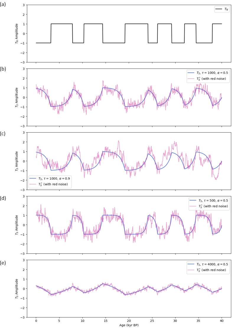
1. Initialization: set default parameter and generate forcing

import numpy as np
import matplotlib.pyplot as plt
from scipy.signal import fftconvolve

class BipolarSeesawModel:
    def __init__(self, tau=1000, dt=50, T_max=40000, alpha=0.6, TN=None):
        self.tau = tau          # Characteristic timescale (years)
        self.dt = dt            # Time step (years)
        self.T_max = T_max      # Simulation length (years)
        self.t = np.arange(0, self.T_max, self.dt)
        self.alpha = alpha      # Red‑noise coefficient
        self.TN = TN if TN is not None else self.generate_tn()  

    def generate_tn(self):
        """Create a stochastic square‑wave (±1) Northern Hemisphere forcing."""
        TN = np.zeros_like(self.t)
        current_state, t_switch = 1, 0
        while t_switch < self.T_max:
            duration = np.random.uniform(2000, 5000)
            next_switch = t_switch + duration
            TN[(self.t >= t_switch) & (self.t < next_switch)] = current_state
            current_state *= -1  # flip polarity
            t_switch = next_switch
        return TN

2. Computing Southern Hemisphere temperature

    def compute_ts_convolution(self):
        """Compute Southern temperature, T_S, via causal convolution."""
        t_prime = np.arange(0, 10 * self.tau, self.dt)
        kernel = np.exp(-t_prime / self.tau) / self.tau
        kernel /= np.sum(kernel * self.dt)                 # to ensure unit area
        TS = -fftconvolve(self.TN, kernel, mode='full')[:len(self.TN)] * self.dt
        self.TS = TS
        return TS

3. Adding autoregressive red‑noise perturbations

    def generate_red_noise(self):
        """Add red noise r(t) = α·r(t−Δt) + ε(t)."""
        red_noise = np.zeros_like(self.TS)
        white_noise = np.random.normal(0, 0.4 * np.std(self.TS), size=len(self.TS))
        for i in range(1, len(self.TS)):
            red_noise[i] = self.alpha * red_noise[i - 1] + white_noise[i]
        self.red_noise = red_noise
        self.TS_noisy = self.TS + red_noise
        return red_noise

4. Simulation, visualization, and scenario choices for example experiments

    def run(self):
        self.compute_ts_convolution()
        self.generate_red_noise()
        return self.TN, self.TS, self.TS_noisy

def run_scenarios(scenarios=None, single_scenario=None):
    TN_fixed = BipolarSeesawModel().generate_tn()

    if single_scenario:
        scenarios = [single_scenario]

    models = [BipolarSeesawModel(tau=sc["tau"], alpha=sc["alpha"], TN=TN_fixed)
              for sc in scenarios]
    results = [model.run() for model in models]

    t = models[0].t
    kyrBP = (models[0].T_max - t) / 1000   # convert to kyr BP for plotting

    fig, axes = plt.subplots(nrows=len(scenarios) + 1,
                             figsize=(10, 3 * (len(scenarios) + 1)),
                             sharex=True)

    axes[0].plot(kyrBP, TN_fixed, 'k', label="$T_N$")
    axes[0].set_ylabel("$T_N$ amplitude")
    axes[0].legend(); axes[0].set_ylim(-3, 3)

    for i, (sc, (_, TS, TS_noisy)) in enumerate(zip(scenarios, results)):
        axes[i + 1].plot(kyrBP, TS, 'royalblue',
                         label=fr"$T_S$, τ={sc['tau']}, α={sc['alpha']}")
        axes[i + 1].plot(kyrBP, TS_noisy, 'mediumvioletred', alpha=0.4,
                         label="$T_S^*$ (with red noise)")
        axes[i + 1].set_ylabel("$T_S$ amplitude")
        axes[i + 1].legend(); axes[i + 1].set_ylim(-3, 3)

    axes[-1].set_xlabel("Age (kyr BP)")
    plt.tight_layout(); plt.show()

run_scenarios(single_scenario={"tau": 1500, "alpha": 0})

scenarios = [
    {"tau": 1000, "alpha": 0.5},
    {"tau": 1000, "alpha": 0.9},
    {"tau": 500,  "alpha": 0.5},
    {"tau": 4000, "alpha": 0.5},
]
run_scenarios(scenarios=scenarios)

Below are the two questions I addressed in the assignment write-up.

Q: Are you impressed by the comparisons to the Byrd ice‑core isotopic data? Why / why not?

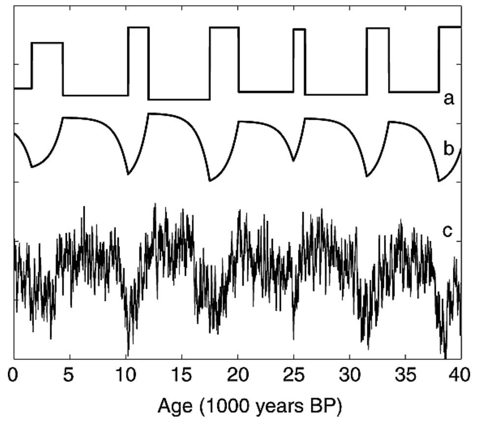
The results are impressive, as the model successfully mirrors nearly all DO events observed in Greenland within the Antarctic record. Even the smaller oscillations associated with less prominent DO events (e.g., 3–7 and 9–11) have corresponding features in model results. Also, the relative amplitude of warm phases in model results closely resembles that of Byrd data, though it slightly underestimates some peaks (e.g., A1 and A2 appear somewhat weaker in c). Some other minor discrepancies include: 1. The Byrd record seemingly exhibits sharper transitions in certain events, whereas the modeled curve appears more smoothed—likely a result of the convolution process; 2. In the earlier part of the record (e.g., 60–65 kyr bp), there are slight timing offsets between model output and Byrd data. Despite these minor limitations, the overall agreement between the modeled and observed Byrd records is remarkable.

Q: SJ03 call theirs the “simplest possible thermodynamic model” of the bipolar seesaw. Which climate processes does it capture, and what is missing?

SJ03 explains the inverse relationship between abrupt North Atlantic cooling and gradual Antarctic warming by modeling the southern heat reservoir as a time-integrated response that smooths and lags Northern Hemisphere climate signals . Their model effectively captures the bipolar seesaw and DO cycles using a simple thermodynamic framework, although there are several simplifications—for instance, it represents temperature changes in the North Atlantic as a “square wave” without addressing the underlying mechanisms that trigger these abrupt shifts. Additionally, while the model identifies an optimal τ (~1120 years) through correlation tests, it does not offer a physical explanation for why this specific timescale emerges.

Thermodynamics is a fundamental component of the climate system, but it does not encompass all relevant processes. As a result, several crucial mechanisms involved in DO cycles are missing from this model. Firstly, while temperature variations can partially reflect AMOC dynamics, AMOC strength is controlled not only by temperature but also by salinity. A more physically complete representation of AMOC variability would require incorporating salinity changes and key drivers like freshwater forcing and sea ice dynamics. This may be achieved by integrating a Stommel two-box model. Other essential climate processes that could be included are: (1) Atmospheric processes, which are influenced by ice sheet height, and play a crucial role in heat transport and wind-driven ocean circulation (Zhang et al., 2014); (2) Ice sheet dynamics and isostatic adjustments, which are critical for the Heinrich events (Bassis et al., 2017); (3) CO₂ forcing and (4) Orbital forcing, which likely control the pacing and magnitude of DO events over longer timescales (Zhang et al., 2017; Hodell et al., 2023).

Reference

Stocker, T. F., & Johnsen, S. J. (2003). A minimum thermodynamic model for the bipolar seesaw. Paleoceanography, 18(4), 1087. https://doi.org/10.1029/2003PA000920